Beyond scRNAseq: neuronal recordings#
In this tutorial we are showing the applicability of scFates on other high-dimensional datasets, such as single neuronal acitvity recordings, in order to extract population dynamics.
The dataset and preprocessing#
In this example we will use data from Peyrache et al, which is a study on mammalian head direction cell recordings. Here is the figure 1 that summaries the location and data recorded:
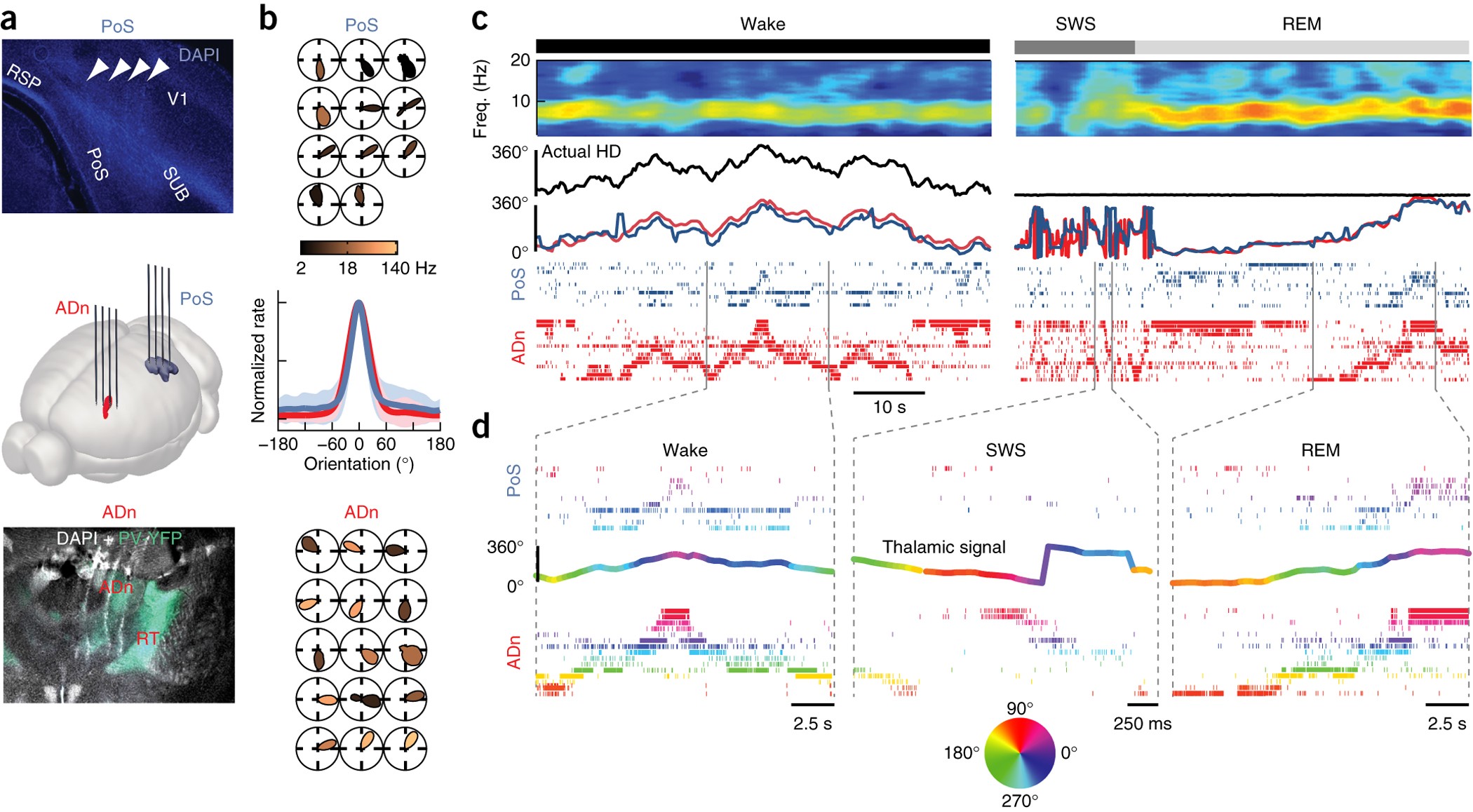
The data used for this tutoral includes recordings from 22 neurons located in the anterodorsal thalamic nucleus (ADn) of a single mouse that was awake and foraging in an open environment, with measured head angles.
Preprocessing#
Following Chaudhuri et al. method, spike times were converted into time-varying rates. Firing rates were estimated by convolving the spike times with a Gaussian kernel of standard deviation 100 ms. The rates were then replaced by their square root to stabilize the variance. For each timepoint is the related measured angle.
Load libraries and data#
[1]:
import pandas as pd
import numpy as np
import palantir
import anndata
import warnings
# ignore all future warnings
warnings.filterwarnings("ignore")
import scFates as scf
import scanpy as sc
import scanpy.external as sce
import seaborn as sns
import matplotlib.colors as col
import seaborn
seaborn.reset_orig()
%matplotlib inline

N = 256
flat_huslmap = col.ListedColormap(sns.color_palette('husl',N))

angle_u = 'https://github.com/LouisFaure/scFates_notebooks/raw/main/data/angles.csv.gz'
counts_u = 'https://github.com/LouisFaure/scFates_notebooks/raw/main/data/counts.csv.gz'
findfont: Font family ['Raleway'] not found. Falling back to DejaVu Sans.
[2]:
counts=pd.read_csv(counts_u,header=None)
counts.index=counts.index.astype(str)
counts.columns=counts.columns.astype(str)
counts.shape
[2]:
(22841, 22)
[3]:
adata=anndata.AnnData(counts)
adata.obs['angles']=np.degrees(pd.read_csv(angle_u, header=None).values)
[4]:
adata.obs['time']=np.arange(0,adata.shape[0]*0.05,0.05)
Dimensionality reduction#
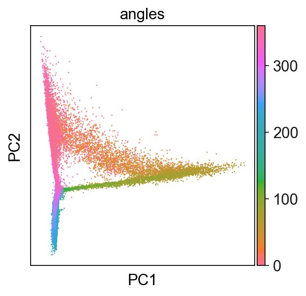
PCA#
[5]:
sc.pp.pca(adata)
[6]:
sc.set_figure_params()
sc.pl.pca(adata,color="angles",cmap=flat_huslmap)
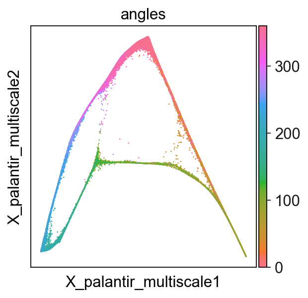
Multi-scale diffusion maps#
[7]:
sce.tl.palantir(adata)
adata
Determing nearest neighbor graph...
[7]:
AnnData object with n_obs × n_vars = 22841 × 22
    obs: 'angles', 'time'
    uns: 'pca', 'palantir_EigenValues'
    obsm: 'X_pca', 'X_palantir_diff_comp', 'X_palantir_multiscale'
    varm: 'PCs'
    layers: 'palantir_imp'
    obsp: 'palantir_diff_op'
[8]:
adata.obsm["X_palantir_multiscale"].shape
[8]:
(22841, 7)
[9]:
sc.pl.embedding(adata,basis='X_palantir_multiscale',color='angles',cmap=flat_huslmap)
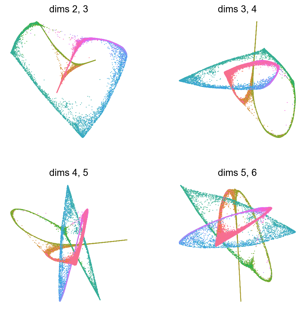
Show several dimensions of multiscale diffusion space#
[10]:
import matplotlib.pyplot as plt
fig, axs = plt.subplots(2,2,figsize=(8,8))
axs=axs.ravel()
for d in np.arange(2,6):
    sc.pl.embedding(adata,basis='X_palantir_multiscale',
                    title="dims %d, %d"%(d,d+1),
                    dimensions=(int(d),int(d+1)),
                    color='angles',cmap=flat_huslmap,
                    show=False,ax=axs[d-2],frameon=False)

    # complex way to remove the side colorbar
    axs[d-2].set_box_aspect(aspect=1)
    fig = axs[d-2].get_gridspec().figure
    cbar = np.argwhere(
        ["colorbar" in a.get_label() for a in fig.get_axes()]
    ).ravel()
    if len(cbar) > 0:
        fig.get_axes()[cbar[0]].remove()
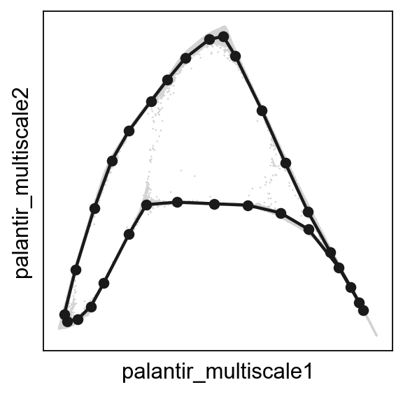
Principal circle fitting#
[11]:
scf.tl.circle(adata,Nodes=30,use_rep="X_palantir_multiscale",device="gpu")
inferring a principal circle --> parameters used
    30 principal points, mu = 0.1, lambda = 0.01
    there are 1 non assigned nodes
    finished (0:00:16) --> added
    .uns['epg'] dictionnary containing inferred elastic circle generated from elpigraph.
    .obsm['X_R'] hard assignment of cells to principal points.
    .uns['graph']['B'] adjacency matrix of the principal points.
    .uns['graph']['F'], coordinates of principal points in representation space.
[12]:
scf.pl.graph(adata,basis='palantir_multiscale')

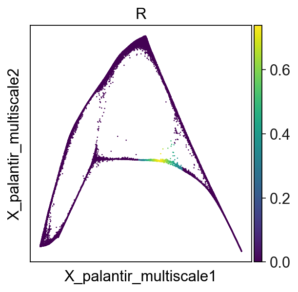
Converting to soft assigment matrix#
ElPiGraph lead to a hard assignment matrix \(R\), rendering it impossible to perform multiple mappings to account for variability, as the assignment to nodes are either 0 or 1:
[13]:
adata.obs["R"]=adata.obsm["X_R"][:,25]
sc.pl.embedding(adata,basis='X_palantir_multiscale',color='R')
To alleviate this limitation, we can apply one iteration of SimplePPT algorithm, generating a soft assignment matrix \(R\), with continuous values between 0 and 1:
[14]:
scf.tl.convert_to_soft(adata,sigma=1,lam=100)
Converting R into soft assignment matrix
    finished (0:00:00) --> updated
    .obsm['X_R'] converted soft assignment of cells to principal points.
    .uns['graph']['F'] coordinates of principal points in representation space.
[15]:
adata.obs["R"]=adata.obsm["X_R"][:,25]
sc.pl.embedding(adata,basis='X_palantir_multiscale',color='R')

[16]:
scf.pl.graph(adata,basis='palantir_multiscale')
Projecting activities over pseudotime#
Select root node characterized by activity at minimum angle#
[17]:
scf.tl.root(adata,root="angles",min_val=True)
automatic root selection using angles values
node 27 selected as a root --> added
    .uns['graph']['root'] selected root.
    .uns['graph']['pp_info'] for each PP, its distance vs root and segment assignment.
    .uns['graph']['pp_seg'] segments network information.
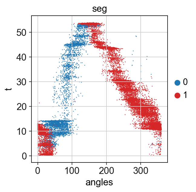
To enable multiple mappings, the circle is considered as a trajectory composed of two segments from the selected root and clostest node converging to the furthest node.
[18]:
scf.tl.pseudotime(adata,n_jobs=50,n_map=50,seed=42)
projecting cells onto the principal graph
    mappings: 100%|██████████| 50/50 [00:58<00:00,  1.16s/it]
    finished (0:01:13) --> added
    .obs['edge'] assigned edge.
    .obs['t'] pseudotime value.
    .obs['seg'] segment of the tree assigned.
    .obs['milestones'] milestone assigned.
    .uns['pseudotime_list'] list of cell projection from all mappings.
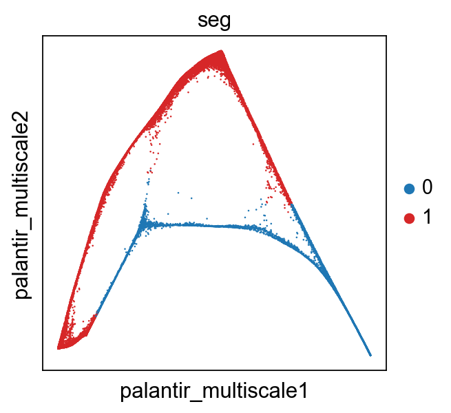
[19]:
sc.pl.scatter(adata,x='angles',y='t',color="seg",palette=["tab:blue","Tab:red"])
sc.pl.embedding(adata,color="seg",basis='palantir_multiscale')
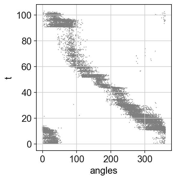
Unroll the circle to get a pseudotime value for all parts of the cicle#
To obtain a pseudotime value that differs between the two segments, one can unroll the circle into a single curved trajectory starting from the root and ending to its closest node.
[20]:
scf.tl.unroll_circle(adata)
--> updated
    .obs['t'] assigned pseudotime value.
    .obs['seg'] assigned segment of the tree.
    .uns['graph']['root'] selected root.
    .uns['graph']['pp_info'] for each PP, its distance vs root and segment assignment.
    .uns['graph']['pp_seg'] segments network information.
[21]:
sc.pl.scatter(adata,x='angles',y='t')
GAM fit of single neuron activities#
[22]:
scf.tl.fit(adata,features=adata.var_names,n_jobs=10)
fit features associated with the trajectory
    single mapping : 100%|██████████| 22/22 [00:25<00:00,  1.15s/it]
    finished (adata subsetted to keep only fitted features!) (0:00:25) --> added
    .layers['fitted'], fitted features on the trajectory for all mappings.
    .raw, unfiltered data.
[23]:
adata.uns["graph"]["milestones"]
[23]:
{'10': 10, '24': 24, '27': 27}
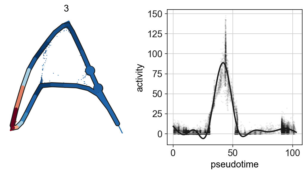
[24]:
scf.pl.single_trend(adata,'3',basis='palantir_multiscale',frameon=False,
                    color_exp="k",alpha_expr=.04,ylab='activity')
[25]:
g=scf.pl.trends(adata,plot_emb=False,highlight_features=[],ordering="max",
              fig_heigth=6,pseudo_cmap=flat_huslmap,ord_thre=.95,return_genes=True)
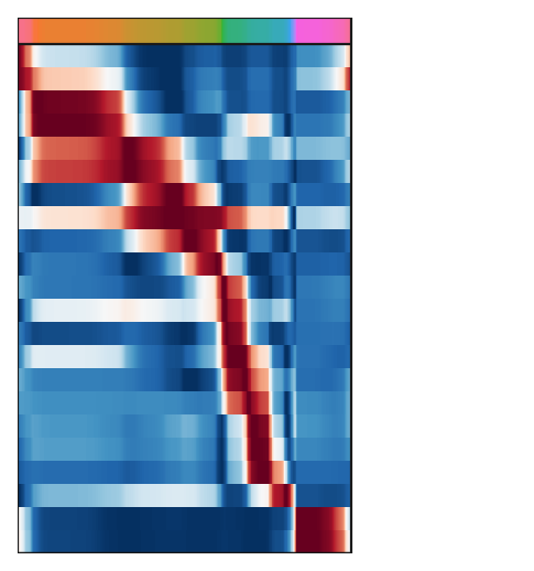
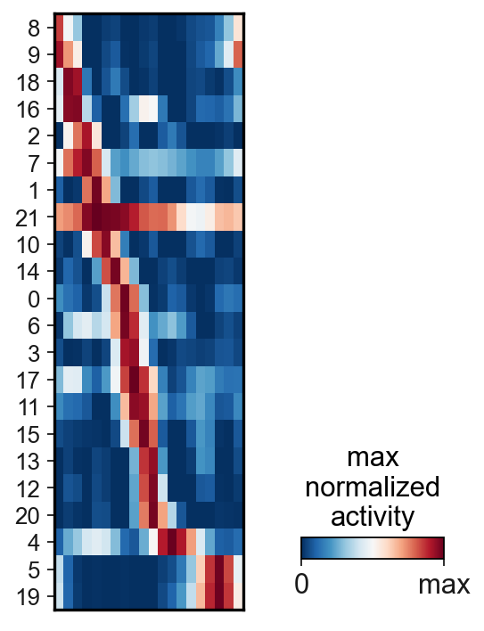
[26]:
scf.pl.matrix(adata,features=g,nbins=20,
              cmap="RdBu_r",annot_top=False,
              colorbar_title="max\nnormalized\nactivity")